Data Analysis 101: My beginner project.

What we'll be doing today.
We will follow these steps on Given Dataset
- Trying to make sense of the data.
- Checking if there's any dirty data.
- Visualizing the clean data.
- Final Conclusion.
Step 1: Understand the data
- First we will load the Data
- We will create a rough Flowchart of Insights we can get from the Data
- Move to next Step
# First of all we'll load all the libraries

import numpy as np
import pandas as pd
import matplotlib.pyplot as plt
import seaborn as sns
Then we'll go ahead and read the source file from which we'ed be getting the data.
You can download the .csv file from here - https://github.com/realharshbhatt/Pythonproject/blob/main/Stores.csv
df=pd.read_csv('/Projects/Stores/Stores.csv')
df.head()
(Note - change the path to where you've stored the .csv file.)
Store ID     Store_Area     Items_Available     Daily_Customer_Count     Store_Sales
0     1     1659     1961     530     66490
1     2     1461     1752     210     39820
2     3     1340     1609     720     54010
3     4     1451     1748     620     53730
4     5     1770     2111     450     46620
Step-2: Data Cleaning
To find the missing and in correct values we generally use 3 Functions
- df.isnull( ).sum( ): It will give you total NULL values in each column
- df.info( ): This is very useful, This will give you all information like 'Non-Null Values' & 'Data Type' for each column
- df.unique( ): Gives you all unique values of a function
df.isnull().sum()
The Output we get would look something like this -
Store ID                0
Store_Area              0
Items_Available         0
Daily_Customer_Count    0
Store_Sales             0
dtype: int64
For more info about the columns, we will use info() function
df.info()
We can see that all the columns data is integer type
<class 'pandas.core.frame.DataFrame'>
RangeIndex: 896 entries, 0 to 895
Data columns (total 5 columns):
 #   Column                Non-Null Count  Dtype
---  ------                --------------  -----
 0   Store ID              896 non-null    int64
 1   Store_Area            896 non-null    int64
 2   Items_Available       896 non-null    int64
 3   Daily_Customer_Count  896 non-null    int64
 4   Store_Sales           896 non-null    int64
dtypes: int64(5)
memory usage: 35.1 KB
Cleaning the individual data.
We will use unique() function to find all the unique values in store area column.
df.Store_Area.unique()
Below we can see all the unique values in the column.
array([1659, 1461, 1340, 1451, 1770, 1442, 1542, 1261, 1090, 1030, 1187,
       1751, 1746, 1615, 1469, 1644, 1578, 1703, 1438, 1940, 1421, 1458,
       1719, 1449, 1234, 1732, 1475, 1390, 1642, 1715, 1439, 1250, 1331,
       1784, 1375, 1871, 1174, 1839, 1270, 1435,  965, 1665, 1780, 1009,
       1227, 1769, 1660, 1472, 1408, 1514, 1565, 1074, 1864, 1570, 1417,
       1734, 1470, 1761, 1756, 1704, 2011, 1310, 1544, 1707, 1881, 1416,
       1631, 1318, 1692, 1152,  891, 1468, 1539, 1635, 1267, 1720, 1462,
       1431, 1441, 1572, 1287, 1931, 1252, 1238, 1479, 1590, 2169, 1838,
       1385, 1921, 1975, 1853, 1816, 1785, 1579, 1096, 1919, 1262, 1374,
       1309, 1207, 1929, 1573, 1415, 1162, 1485, 1897, 1607, 1909, 1274,
       1157, 1712, 1500, 1682, 1525, 1947, 1164, 1787, 1718, 1365, 1368,
       1342, 1076, 1396, 1713, 1370, 1667, 1638, 1581, 1795, 1179, 1978,
       1688, 1214, 1504, 1498, 1229, 1936, 1369, 1662, 1548, 1649, 1393,
       1450, 1613,  775, 1275, 1740, 1372, 1414, 2044, 1823,  955, 1465,
       1232, 1481, 1343, 1007, 1762, 1527, 1356, 1536, 1605, 1626, 1612,
       1923, 1702, 1398, 1437, 1524, 1302, 1666, 1391, 1778, 1652, 1841,
       1496, 1148, 1321,  992, 1540, 1807, 1526, 1406, 1575, 1488, 1658,
       1863, 1604, 1620, 1251, 1647, 1829, 1852, 1699, 1325, 1350, 1347,
       1397, 1245, 1366, 1378, 1767, 1184, 1257, 1329, 1557, 2007, 1185,
       1657, 1294, 1296, 1733, 1641, 1373, 1550, 1583, 1428, 1648, 1025,
       2001, 1145,  913, 1199, 1875, 1153, 1240, 1381, 1701, 1206, 1476,
       1189, 1837, 1319, 1617, 1517, 1764, 1855, 1327, 1533, 1856, 1000,
       1313, 1494, 1386, 1979, 1057,  902, 1314, 1513, 1305, 1180, 1142,
       1471, 1075, 1585, 1577, 1092, 1523, 1614, 1566, 2019, 1766, 1293,
       1236, 1332, 1208, 1190, 1448, 1771, 1510, 1808, 1640, 1060, 1633,
       1222, 1619, 1624, 1887, 1320, 1455,  966, 1922, 1678, 2004, 1954,
       1362, 1886, 1291, 1584, 1445, 1433, 1269, 1798, 1015, 1495, 1759,
       1219, 1571, 1404, 1124, 1484, 1111, 1078, 1876, 1412, 1121, 1691,
       1599, 1454, 1555, 1554, 1491, 1487, 1339, 1509, 1264, 1905, 1209,
       1546, 1689, 2063, 1848, 1480, 1576, 1948,  896, 1625, 1303, 1410,
       1432, 1891, 1322, 1440, 1280, 1161, 1175, 1395, 1443, 1247, 1788,
       1138, 1709, 1777, 1618, 1311, 1249, 1744, 1297, 1908, 1721, 1243,
       1307, 1628, 1556, 1768, 1685, 1474, 1794, 1086, 1501, 1353, 1165,
       1845, 1172, 1436, 1738, 2229, 1490, 2015, 1611, 1430, 1543, 1836,
       1463, 1213, 1244, 1745,  933, 1675, 1842, 1316, 1760, 1323, 1230,
       1167, 1429, 1609, 1109, 1191, 1335, 1382, 1588, 1918, 1334, 1832,
       1271, 1735, 1627, 1351, 1520, 1537, 1622, 1001, 1857, 1552, 1700,
       1482, 1192, 1601, 2214, 1141,  869, 2049, 1883, 1723,  932, 1137,
       1231, 1237, 1371, 1748, 1212, 1466, 2026, 1772, 1511, 1834, 1143,
       1586, 1860, 1424, 1710, 1553, 1814, 1847,  946, 1563, 1664, 1241,
       1690, 1289, 1608, 1344, 1529, 1677, 1426, 1503, 1971, 1383, 1508,
       1411, 1545, 1505, 1422, 1564, 1568, 1933, 1593, 1812, 1580, 1100,
       1534, 1299, 1989, 1809, 1193, 1348, 1132, 1427, 1211, 1717, 1068,
       1755, 1591, 1797, 1519, 1637, 1203, 1884, 1160, 1317, 1560, 1645,
       1225, 1655, 1872, 1434, 1791, 1693, 1502, 1360, 1246, 1990,  967,
       1582, 1827, 1118, 1799, 1493, 1033, 1854, 1937, 1743, 1098, 1358,
       1336, 1418,  854, 1361, 1085, 1453, 1389, 1486, 1464, 1197, 1878,
       1150, 1562, 1596, 1119, 1116, 1934, 1235, 1497, 1444, 1477, 1041,
       1226, 1489, 1549, 1073, 1473, 2013, 1561, 1574, 1388, 1349, 1862,
       1200, 1722, 1850, 1447, 1679,  994, 1354, 1597, 1873, 1218, 1822,
       1716, 1072, 1330, 1425, 1363, 1671, 1379, 1724,  986, 1651, 1916,
       1528, 1409, 1419, 1535,  919, 2067, 1977, 1653, 1939, 1846,  780,
       1775, 1800, 1859, 1259, 1205, 1792, 1263, 1819, 1357, 1156, 1387],
      dtype=int64)
Nothing looks out of place, so now we can move ahead to create a visualization out of it. But before we move forward, if you'd like you can go through the articles that i've attached below if you want to know more details about data cleaning.
Complete Guide to Data Cleaning with Python - (https://medium.com/analytics-vidhya/complete-guide-to-data-cleaning-with-python-8c686104686c)
Data Cleaning with Python - (https://medium.com/bitgrit-data-science-publication/data-cleaning-with-python-f6bc3da64e45)
Ok then, let's get moving, shall we..!
Step-3: Data Visualization
Let's begin with getting a glimpse of how many columns we have to work with.
df.columns
This will show us the Titles of all the columns in our data set.
Index(['Store ID ', 'Store_Area', 'Items_Available', 'Daily_Customer_Count',
       'Store_Sales'],
      dtype='object')
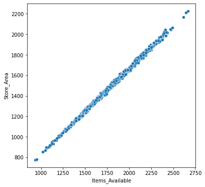
Now let's make our 1st Viz. Trying to find the relation between Store ares and Items available in the store.
plt.figure(figsize=(6,6))
sns.scatterplot(x='Items_Available',y='Store_Area', data=df)
Here we can see that there's a clear co-relation between store area and number of items available.
 You can create various different types of graphs using seaborn library, some of those graph types are:-
- Heatmap
- Histogram
- Bar Plot
- CatPlot (Categorical Plot)
- Density Plot
- Joint Distribution Plot
To know more about types of graphs, you can go through this article:- (https://towardsdatascience.com/14-data-visualization-plots-of-seaborn-14a7bdd16cd7)
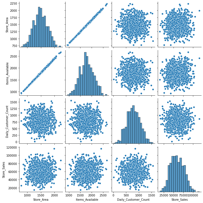
To Plot multiple graph at once, we use pairplot
df1=df
df1.drop(['Store ID '],axis=1,inplace=True)
plt.figure(figsize=(6,6))
sns.pairplot(df1)
From the graphs shown below, we can tell that there is no direct relation between any other Parameter other than store area and items available.
If you want to learn more about creating visualization using seaborn, you can check out this article that explains viz creating using seaborn in detail using Pokemon dataset:- (https://elitedatascience.com/python-seaborn-tutorial)
This was a basic Data Analysis project i made to help me get familiar with the basics.
Thank You!
Comments
Join the discussionNo comments yet. Be the first to comment.